(Task 5) Path Tracing (EXTRA CREDIT)

Up to this point, your renderer simulates light which begins at a source, bounces off a surface, and hits a camera. However in the real world, light can take much more complicated paths, bouncing of many surfaces before eventually reaching the camera. Simulating this multi-bounce light is referred to as indirect illumination, and it is critical to producing realistic images, especially when specular surfaces are present. In this task you will modify your ray tracer to simulate multi-bounce light, adding support for indirect illumination.

You must modify Pathtracer::trace_ray to simulate multiple bounces. We recommend using the Russian Roulette algorithm discussed in class.

The basic structure will be as follows:

• (1) Randomly select a new ray direction using bsdf.sample (which you will implement in Step 2)
• (2) Potentially terminate the path (using Russian roulette)
• (3) Recursively trace the ray to evaluate weighted reflectance contribution due to light from this direction. Remember to respect the maximum number of bounces from max_depth (which is a member of class Pathtracer).

Step 2

Now, Implement BSDF_Lambertian::sample for diffusely reflecting, which randomly samples from the distribution and returns a BSDF_Sample. Note that the interface is in rays/bsdf.h. Task 6 contains further discussion of sampling BSDFs, reading ahead may help your understanding. The implementation of BSDF_Lambertian::evaluate is already provided to you.

Note:

• Functions in student/sampler.cpp from class Sampler contains helper functions for random sampling, which you will use for sampling. Our starter code uses uniform hemisphere sampling Samplers::Hemisphere::Uniform sampler(see rays/bsdf.h and student/sampler.cpp) which is already implemented. You are welcome to implement Cosine-Weighted Hemisphere sampling for extra credit, but it is not required. If you want to implement Cosine-Weighted Hemisphere sampling, fill in Hemisphere::Cosine::sample in student/samplers.cpp and then change Samplers::Hemisphere::Uniform sampler to Samplers::Hemisphere::Cosine sampler in rays/bsdf.h.

---

After correctly implementing path tracing, your renderer should be able to make a beautifully lit picture of the Cornell Box. Below is the rendering result of 1024 sample per pixel.

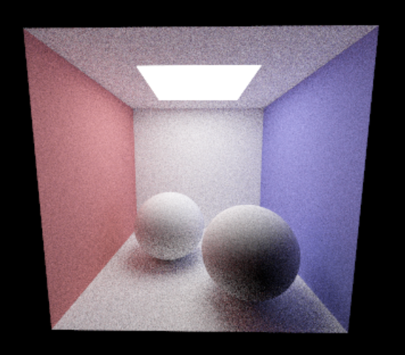
Note the time-quality tradeoff here. With these commandline arguments, your path tracer will be running with 8 worker threads at a sample rate of 1024 camera rays per pixel, with a max ray depth of 4. This will produce an image with relatively high quality but will take quite some time to render. Rendering a high quality image will take a very long time as indicated by the image sequence below, so start testing your path tracer early! Below are the result and runtime of rendering cornell box with different sample per pixel at 640 by 430 on Macbook Pro(3.1 GHz Dual-Core Intel Core i5).

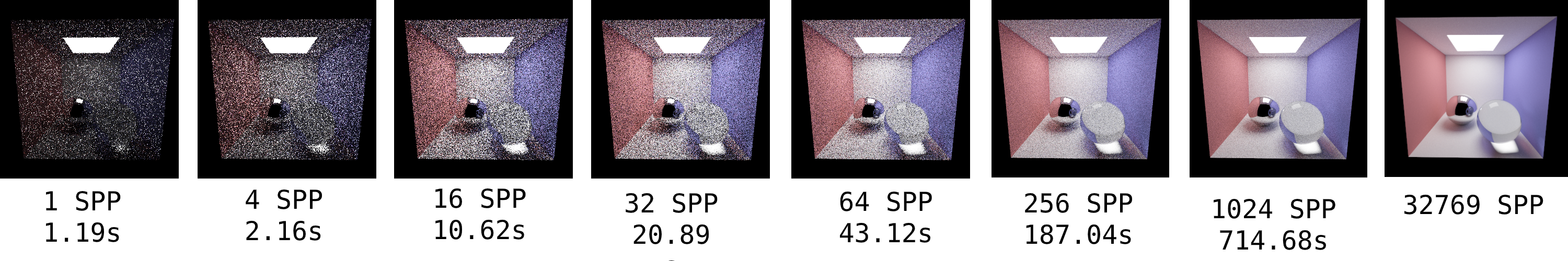
Also note that if you have enabled Russian Roulette, your result may seem noisier.

Here are a few tips:

• The termination probability of paths can be determined based on the overall throughput of the path (you’ll likely need to add a field to the Ray structure to implement this) or based on the value of the BSDF given wo and wi in the current step. Keep in mind that delta function BSDFs can take on values greater than one, so clamping termination probabilities derived from BSDF values to 1 is wise.

• To convert a Spectrum to a termination probability, we recommend you use the luminance (overall brightness) of the Spectrum, which is available via Spectrum::luma

Extra Credit Ideas

• Implement Cosine-Weighted hemisphere sampling to reduce variance in your Monte-Carlo estimates